In this guide, you’ll learn how to sort your data in Google Sheets while keeping the rows together. I will mention two simple methods to accomplish this.
The first method should be used if you want to sort the data in a column just once. If you want to regularly sort any data in a column, I suggest you follow the second method.
For this tutorial, I will use the following sample data as an example, sorting the “Sales” column from the table:
| Order ID | Product Name | Customer Name | Order Date | Sales |
| 1001 | Running Shoes | John Smith | 2024-03-15 | $79.99 |
| 1004 | Protein Powder | David Kim | 2024-03-22 | $49.99 |
| 1006 | Dumbbells | Emily Garcia | 2024-03-19 | $39.99 |
| 1002 | Yoga Mat | Jane Doe | 2024-03-20 | $24.95 |
| 1005 | Baseball Cap | Michael Brown | 2024-03-18 | $19.99 |
| 1003 | Water Bottle | Sarah Lee | 2024-03-12 | $14.50 |
Sorting Once: Using the Sort Function
To sort in Google Sheets and keep rows together using the sort function:
1. Select the data range.
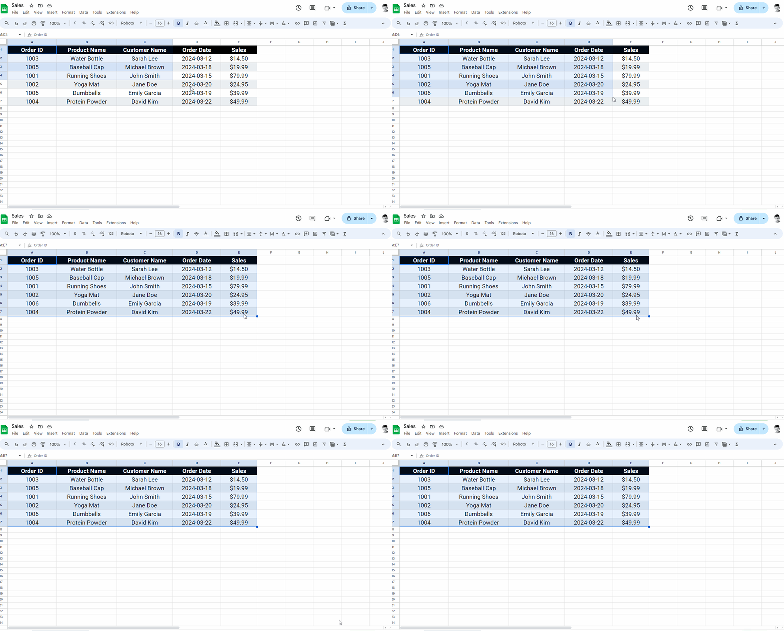
The first step is to select and highlight all the data that you want to sort.
In my case, I selected the entire table.
2. Navigate to Data > Sort range > Advanced range sorting options.
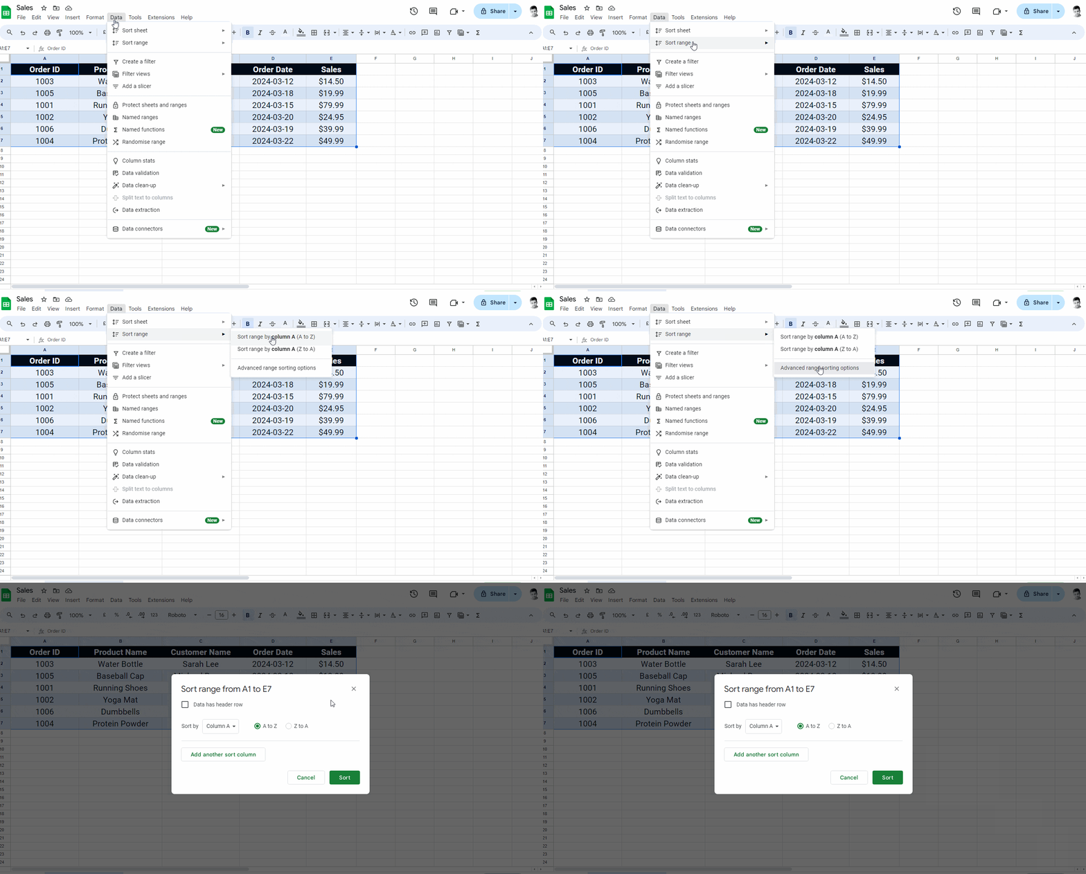
After selecting the data, click on the “Data” option from the top menu.
A menu with a list of options will appear.
Hover over the “Sort range” option to view the secondary menu.
Choose the “Advanced range sorting option” and proceed to the next step.
3. Check the “Data has header row” checkbox.

You will see a pop-up window.
Check the “Data has header row” box if your selected data range includes a header row.
If you don’t have a header row, you can skip this step.
4. Select the column you want to sort.
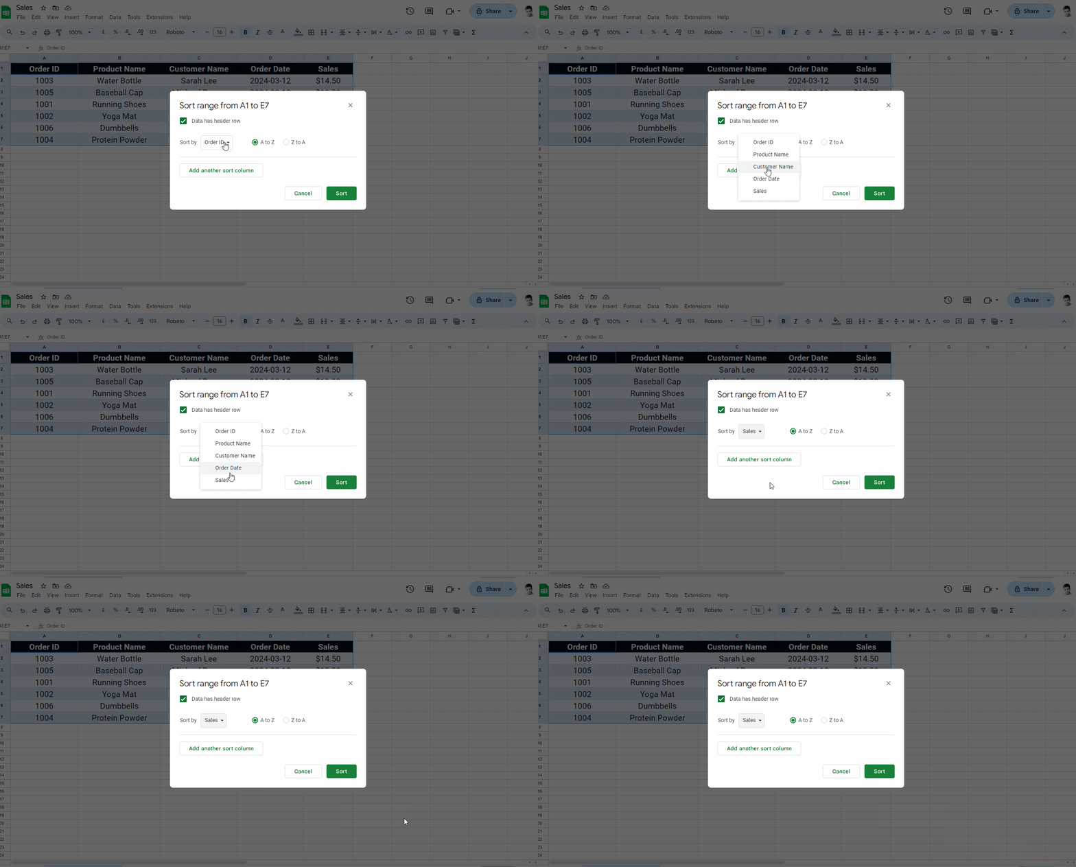
In the “Sort by” drop-down, the first column will be automatically selected.
Click on this drop-down menu and choose the column from the drop-down that you want to sort.
In my case, the “Order ID”, which is the first column, was selected by default.
Since I wanted to sort the “Sales” column, I clicked on the “Sort by” drop-down menu and chose the “Sales” column from the list.
5. Choose a sorting criteria and click “Sort”
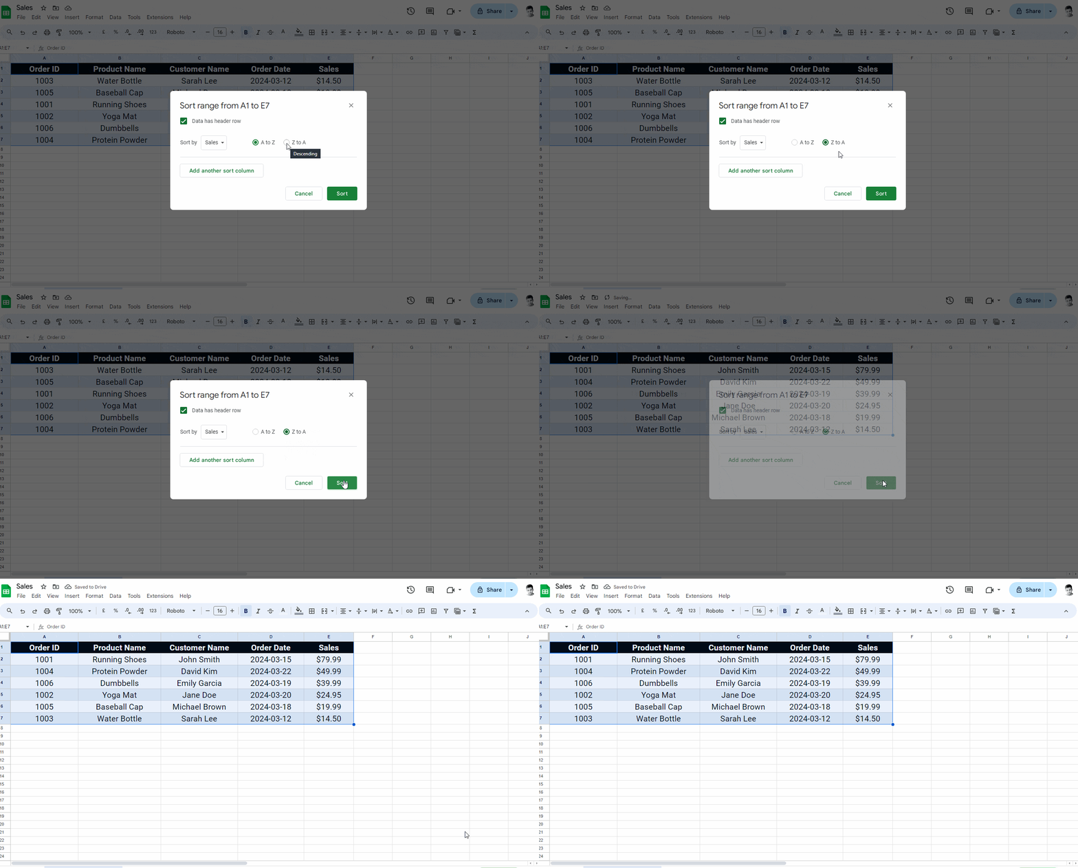
After selecting the column, it is finally time to choose a sorting criterion.
You can either choose to sort the data in an ascending manner (A to Z) or choose the descending option (Z to A).
Now, click the “Sort” button.
Following these five steps every time can be a tedious task, especially if you are working with thousands of rows and columns and you often want to sort columns.
That’s why I have found a way to quickly sort any column from the table in ascending or descending order.
I have explained the method step-by-step in the section below.
Sorting Regularly: Using Filters
To sort in Google Sheets and keep rows together using filters:
1. Select the data range.
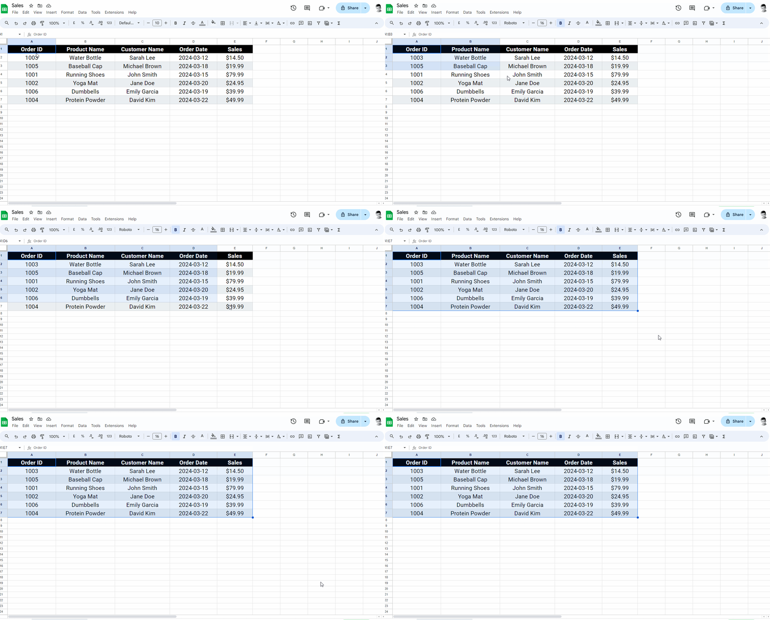
To begin, highlight all the data with the mouse to select it. Now, proceed to the next step.
2. Navigate to Data > Create a filter.
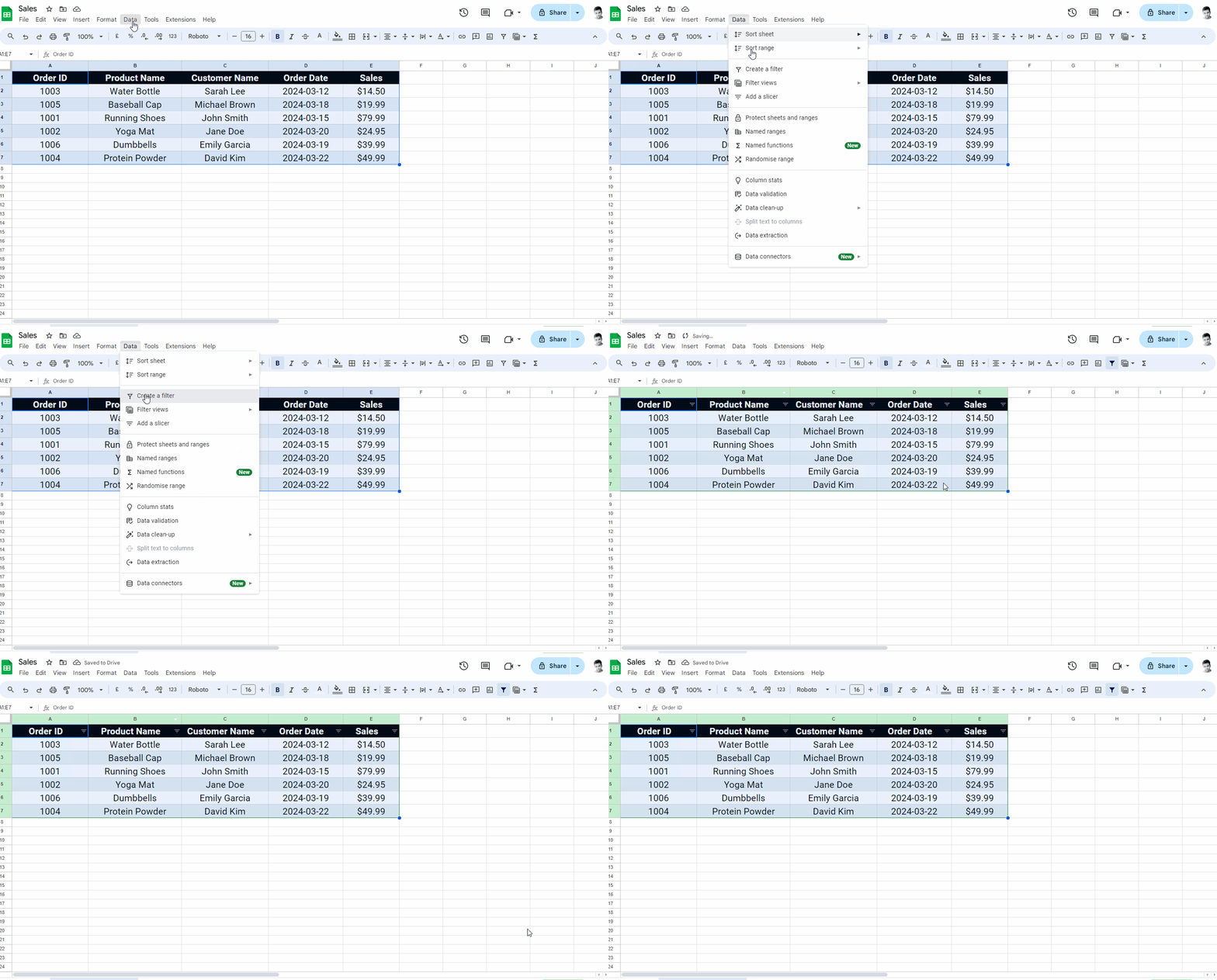
After you select the data, click on the “Data” option from the top menu, then select the “Create a Filter” option from the list of options.
3. Click anywhere on the screen to deselect the data range.

To deselect the data range, simply click anywhere on the sheet. This is an optional step.
4. Click on the filter icon (a downward-facing triangle).
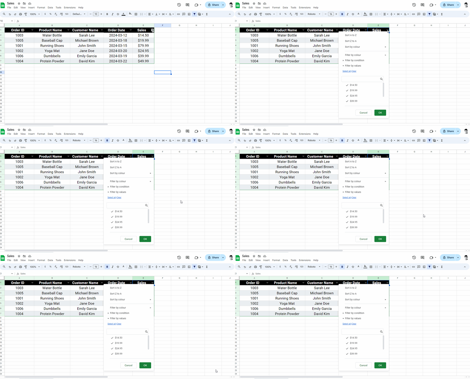
You will now see a filter icon next to each column header. Simply click on it to view the options.
5. Choose a sorting criteria.
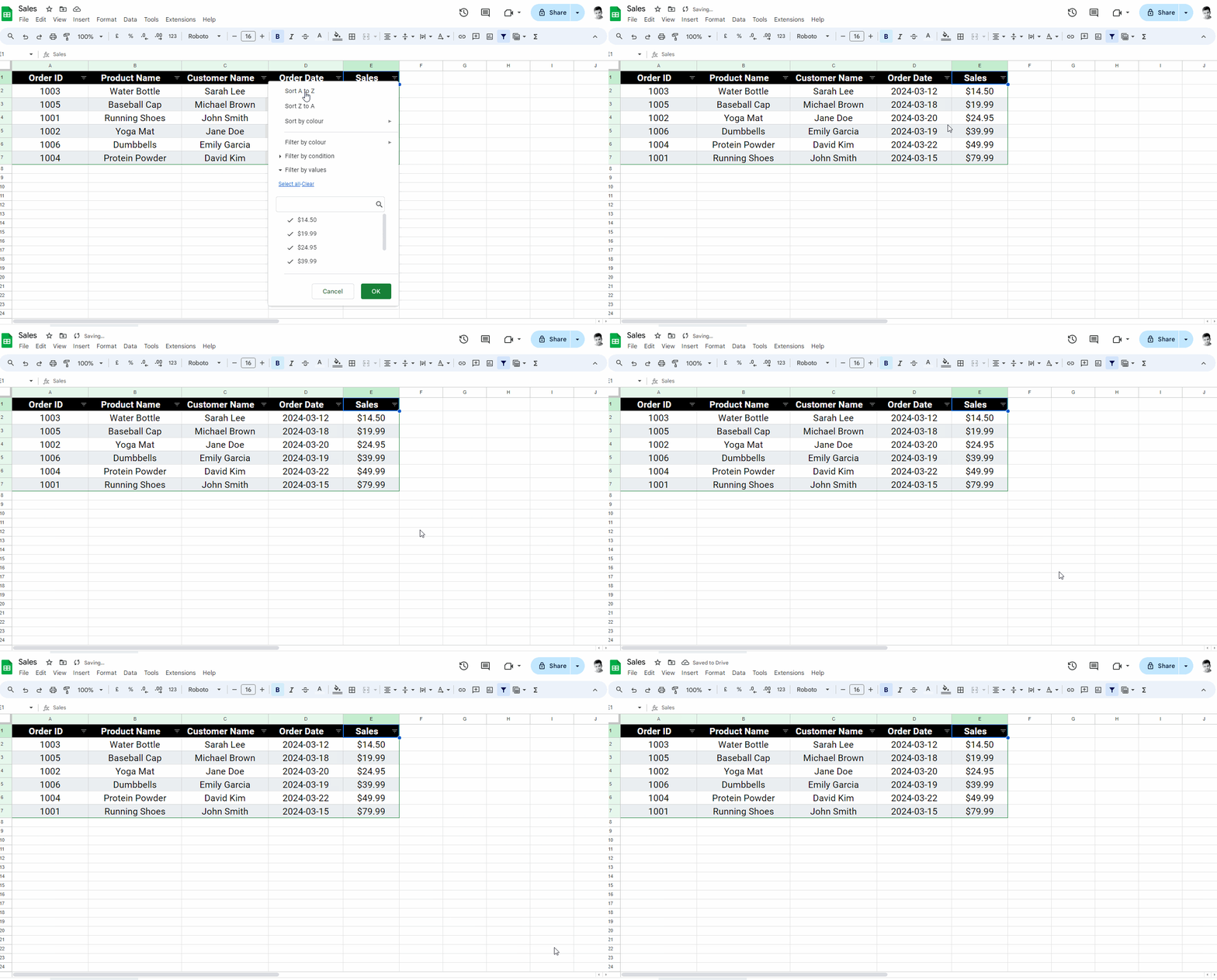
After you click on the filter icon, you will see a menu with options like Sort A to Z, Sort Z to A, and Sort by color.
Choose your desired sorting criteria for the column.
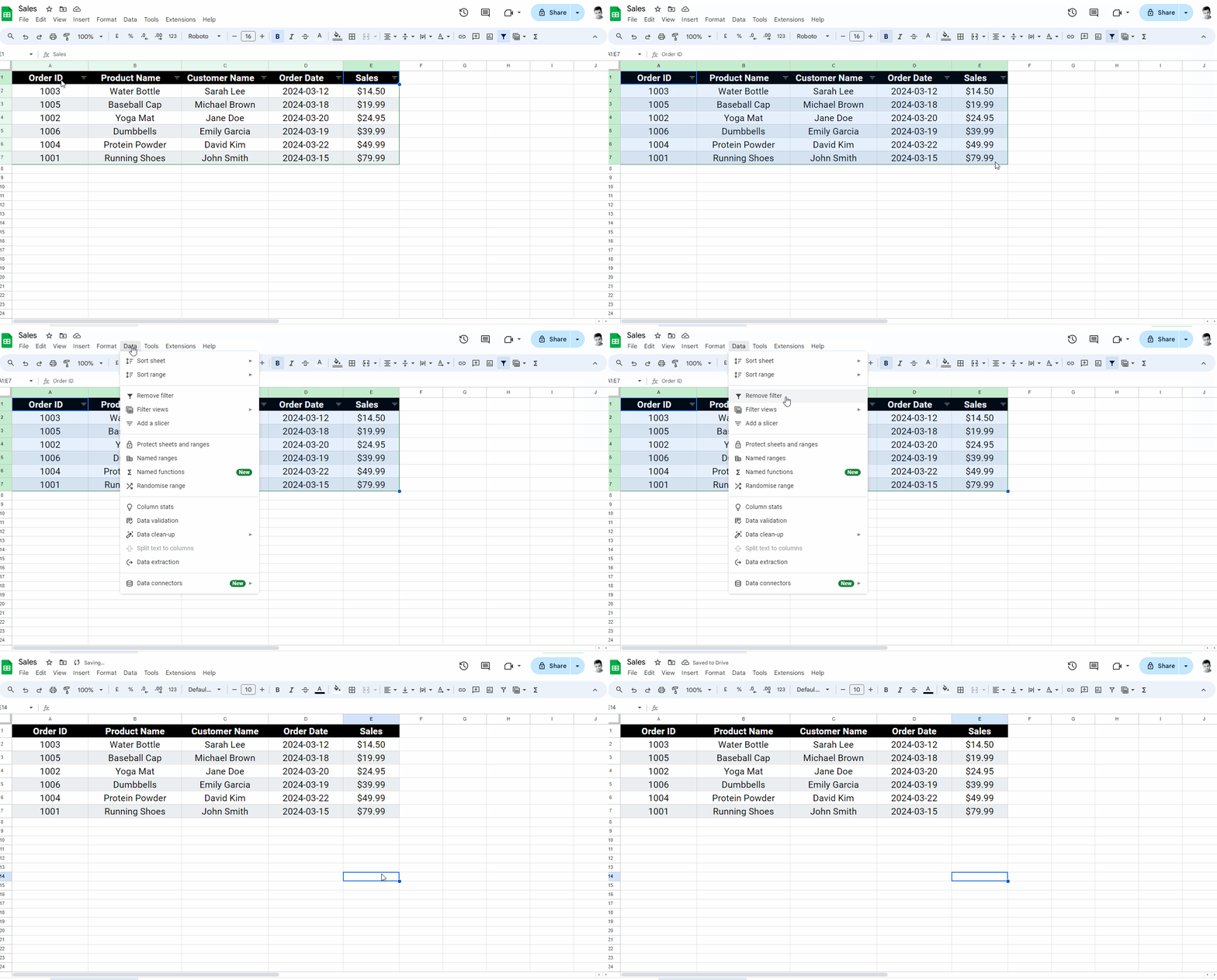
To remove the filter icons, select the entire data range, go to the Data menu, and select “Remove filter”.
